Regularisation: the strange secret behind deep learning
I am probably not alone in finding regularisation to be an almost bizarre concept when first introduced. Why would you artificially penalise your models in ways that don’t benefit the learning task? Adding an L2 term guarantees the final model will walk uphill from its otherwise optimal solution, which seems contrary to the main goal. Subjecting your model to dropout artificially strips elements of its calculation away while it works, forcing it to recover from missing information. These seemingly strange ideas are not just useful hacks that happen to work, but are actually essential to the field of deep learning. Let’s explore why and how in this post.
 A depiction of a scientist “boxing in” their hypothesis class. Generated by ChatGPT 4o
What is regularisation
At its heart the idea of machine learning (ML) can be made quite simple. Taking the case of supervised learning, the process involves creating a network capable of representing a large variety of functional forms through tuning parameters, and then exposing the network to many examples which forces it to become a better match for the exact function we want to find. While ML is a broad field of study, the “search through a function space” concept is general enough to match many of its goals and techniques. This is partly due to an enormous generality of the idea of a function. For example, predicting which word to say next based on the previous 1000 words can be thought of as a function, or stating whether 100x100 pixels show a dog or a cat is another function.
The key to the function search is backpropagation, which is in essence just the ability to take derivatives within a neural network. We choose a loss (or cost) function which decreases as we get closer to the goal, and then check how much the loss function would change if this parameter or that parameter were slightly higher. Repeat that for all parameters, many times over with many different examples and you have a typical ML problem, especially in the context of deep learning (DL).
It can be enormously surprising in this view that once you have chosen a good loss function for a problem you would add a new term which penalises, say, the total magnitude of model parameters. Concrete examples will be given below, but for now we define some useful notation. Consider \(f_{\boldsymbol{\theta}}\) be a neural network governed by parameter vector \(\boldsymbol{\theta}\), and let \((x,y)\) be a single supervised example. For a specific task we use a loss function \(\ell\) which compares values in the output space, so specifically we evaluate \(\ell\big(f_{\boldsymbol{\theta}}(x), y\big)\), which generally approaches zero when \(f_{\boldsymbol{\theta}}(x) \approx y\). In this sense the loss function matches the prediction problem at hand. To differentiate notation we will also write the loss as a function of model parameters \(\mathcal{L}=\mathcal{L}(\boldsymbol{\theta})\). Various types of regularisation consist of adding a new term \(\mathcal{L}_{\rm reg}\), which does not correlate at all with the prediction goal, and often just penalise the network based on its parameters: \(\mathcal{L}_{\rm reg}(\boldsymbol{\theta})\). This forces the model to roll slightly uphill from its otherwise optimal prediction, which is initially very strange in the context of supervised learning.
Other types of regularisation are also strange at first, one example being dropout. This is not applied at the loss level, but instead is part of the model architecture. At training time a dropout layer will randomly zero out some activations with a probability \(0\leq p < 1\). This essentially forces the model to fit a function where certain intermediate values are randomly stripped away from it, therefore making its fitting task far more difficult.
So why do we punish the network in such strange ways while it tries to fit our data? The answer is that while doing so typically sacrifices performance on the training set, it is designed to increase performance on the validation set. In other words, regularisation improves generalisation of the model. How exactly this happens is quite subtle, and requires careful explanation in each case. It can however be very easily shown with experiments, which is where we will start in this post.
Experimental setup
Regularisation can be visualised in even very simple setups, which enables exploration within ML without large datasets and compute budgets. I would strongly advocate for readers to play around with ideas on toy problems. I certainly came away from writing this post with a much better understanding of ML, and some rules learned here have already impacted my work on large real-world data.
The set up I considered was a simple linear regression problem where the data is generated from a vector of true weights \(\boldsymbol{w}\) and a single bias \(b\), with some added Gaussian noise \(\mathcal{N}(0, 1)\) scaled by \(\epsilon\):
\[ y = \boldsymbol{w} \cdot \boldsymbol{x} + b + \epsilon \, \mathcal{N}(0, 1). \]
The weights (and \(\boldsymbol{x}\)) are 50-dimensional, and epsilon is set to \(0.2\). All numbers are chosen at random.
Remark:
When running these tests it is incredibly helpful to reset seeds before doing anything that involves random choices. In this task that means in choosing true weights, bias and noise, in initializing the model, and in the shuffle of data sampling within training.
For this project I found the following code snippet to be sufficient, however the topic can go much deeper:
def reset_seeds(seed=42):
    torch.manual_seed(seed)
    torch.cuda.manual_seed(seed)
    np.random.seed(seed)
In order to get interesting training behaviour in such a simple system we need to train on very few samples, in this case 200. The validation size is set to 10,000 since this does not affect training, but removes any statistical fluctuations from the validation loss. A general strategy in this exploration is to have very low learning rate and many epochs. This is inefficient but yields stable dynamics in training which allow us to study the evolution of model parameters in a smooth way.
Code snippets in the following sections will give necessary hyperparameters to reproduce this work, however the larger functions they allude to are presented in the appendix. I also provide a public repository here. Note that the training loop is designed to be versatile, with more options than are used in this post. That turned out to be incredibly helpful in early testing, and I would encourage others to have a relatively basic yet versatile loop like this saved somewhere for any future projects.
Benchmarks
Given the data we’re modeling, the obvious choice is to perform simple linear regression on the data, although due to the noise added to the labels this will still result in a non-zero final loss. Despite this the final weights found by the network will be unbiased estimators of the true weights mentioned above. Using PyTorch we construct a model with a single linear layer, which we wrap in a class for continuity to other models and to add some helper functions.
class SimpleLinear(torch.nn.Module):
    def __init__(self, in_features, out_features, bias=True):
        super(SimpleLinear, self).__init__()

        # Set seed for reproducibility
        reset_seeds()

        self.linear = torch.nn.Linear(in_features, out_features, bias=bias)

    def forward(self, x):
        return self.linear(x)

    def get_weights(self):
        return self.linear.weight.clone().cpu().detach().numpy().flatten()

model = SimpleLinear(in_features=50, out_features=1).to(device)
Training this model serves as a useful benchmark for what performance is possible on this task.
linear_regression_histories = training_loop(
    model,
    train_dataset,
    val_dataset,
    num_epochs=500,
    lr=0.1,
    device=device
)
plot_training_visualisation(
    linear_regression_histories,
    alpha=0.2,
    savename="linear_benchmark.png"
)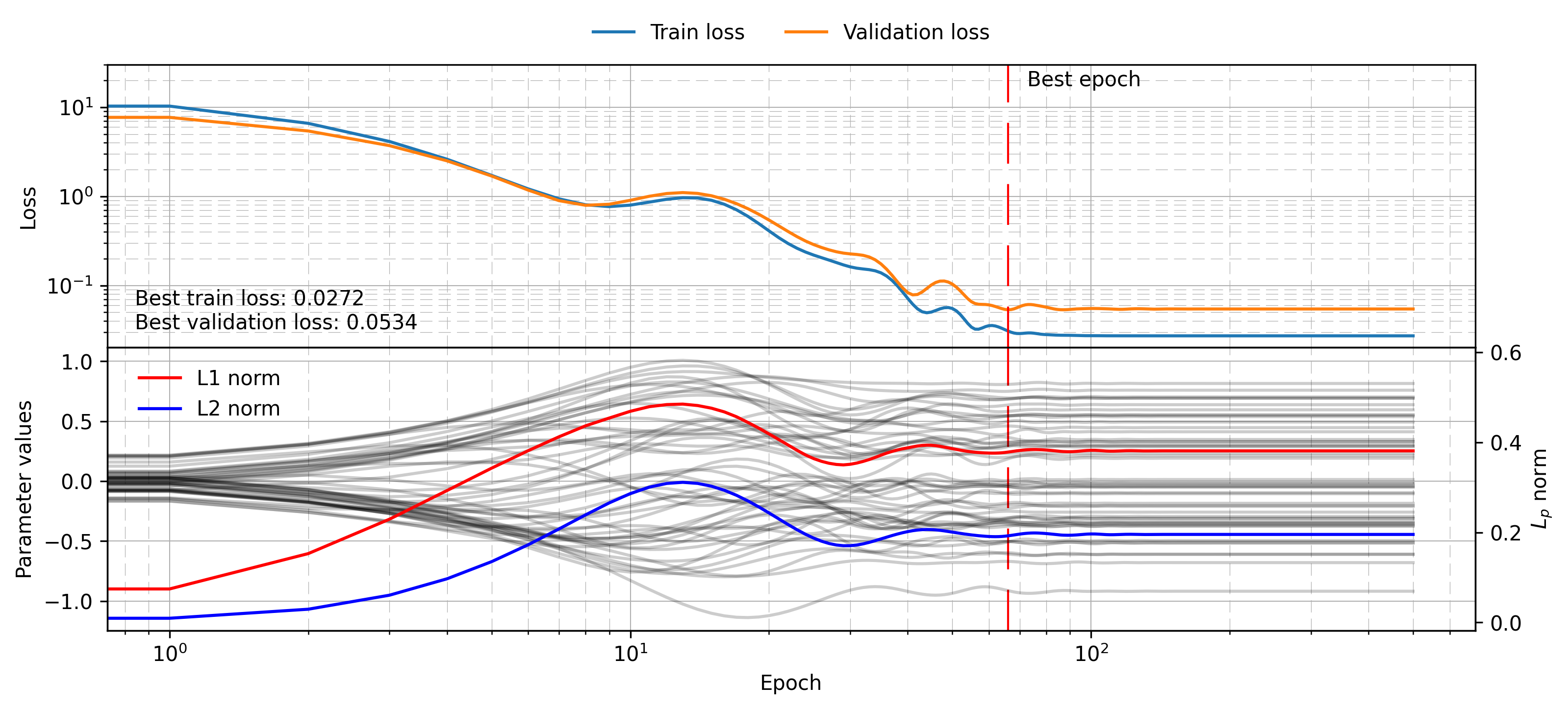
This plot is a bit busy, and will be used throughout the post, so it is worth pausing to analyse it. The top panel shows the training and validation loss over each epoch. The best epoch (as measured by validation loss) is shown with a red dashed line. The value of each parameter is shown in faint black lines in the panel below (left y-axis), while the L1 and L2 norms for the parameter vector are shown in red and blue respectively (right y-axis). The norms will become important as we add regularisation terms to the model. Note that in this case the model is simple enough that the norms naturally evolve over time as the parameters find their appropriate values.
Now we will benchmark a multi-layer perceptron (MLP) model which involves hidden layers and non-linearities. This is not required to fit the data well due to the simplicity of the experiment, but in general non-linearities are needed to fit arbitrary data (see previous post which discusses the universal approximation theorem). The definition of the model is given below, again adding in a helper function for getting model parameters:
class MLP(torch.nn.Module):
    def __init__(self, layer_sizes, activation=torch.nn.ReLU, dropout=0):
        super(MLP, self).__init__()

        # Set seed for reproducibility
        reset_seeds()

        self.layers = torch.nn.ModuleList()

        for i, (l1, l2) in enumerate(zip(layer_sizes[:-1], layer_sizes[1:])):
            self.layers.append(torch.nn.Linear(l1, l2))
            if i < len(layer_sizes)-2:
                self.layers.append(torch.nn.Dropout(dropout))
                self.layers.append(activation())

    def forward(self, x):
        for layer in self.layers:
            x = layer(x)
        return x

    def get_weights(self):
        return np.hstack([p.data.clone().cpu().detach().numpy().flatten() for p in self.parameters()])

model = MLP([50, 25, 25, 1]).to(device)
Note also that this model can now take dropout as a parameter, a regularisation technique we will discuss in the following section. This model now has much more modeling power, which in this experiment means the ability to model the noise added on each label. The results of a simple training loop are shown below:
model = MLP([50, 25, 25, 1]).to(device)
mlp_histories = training_loop(model, train_dataset, val_dataset, num_epochs=1_000, lr=0.01, device=device)
plot_training_visualisation(mlp_histories, savename="mlp_benchmark.png")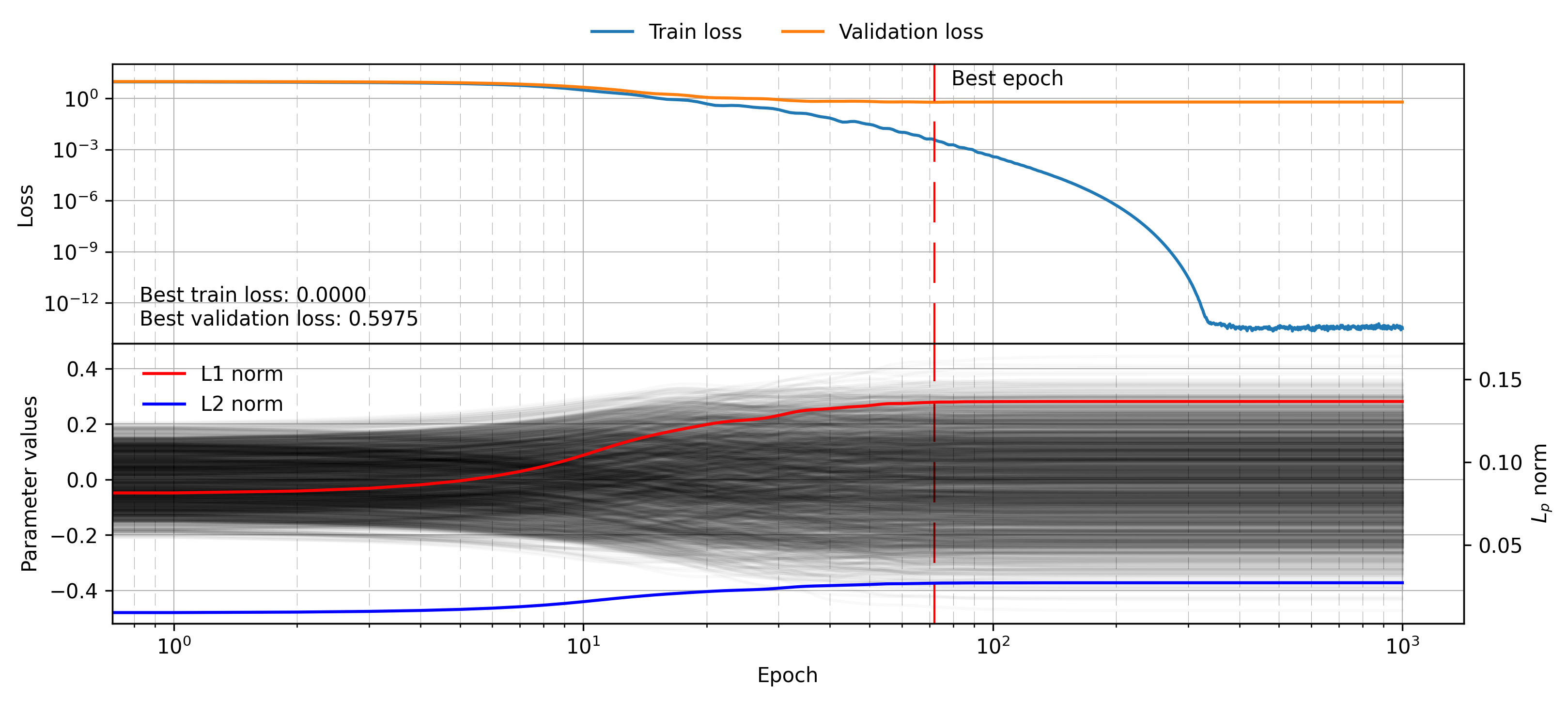
This time the top panel has a very unhelpful scale, because the training loss simply drops to a minimal value which exhibits a lot of numerical noise, likely due to the limits of float32 precision. The validation loss stops improving as this “noise fine-tuning” stage begins, and the final value is much worse than for the linear model (0.60 vs. 0.05). This exemplifies the effect of choosing a much larger hypothesis class than we can afford to search given the samples available to us.
In the following section we will show how regularisation attempts to mitigate effects of overfitting, keeping in mind the worst and best case scenarios for validation loss (0.60 and 0.05 respectively).
Regularisation terms
Weight decay (L2 regularisation)
Probably one of the most common types of regularisation is weight decay, which consists of adding the L2 norm of all model parameters to the loss function weighted by some parameter \(\lambda\). This encourages the model to fit the data without relying on ever larger weights. Concretely the regularisation term takes the form
\[ \mathcal{L}_{L2} = \frac{\lambda}{2}\boldsymbol{\theta}^2 = \frac{\lambda}{2} \sum_i \theta_i^2 \]
which has a gradient
\[ \nabla_{\theta_i} \mathcal{L}_{L2} = \lambda \,\theta_i. \]
This means the parameter update \(\theta_i \leftarrow \theta_i - \eta\,\nabla_{\theta_i}\mathcal{L}\) with learning rate \(\eta\) will tend to decrease each parameter with a force proportional to the value itself. Before discussing why this works, let’s verify that it does indeed improve the networks generalisability.
model = MLP([50, 25, 25, 1])
mlp_weight_decay_histories = training_loop(
    model,
    train_dataset,
    val_dataset,
    num_epochs=1_000,
    lr=0.01,
    weight_decay=0.085,
    device=device
)
plot_training_visualisation(mlp_weight_decay_histories)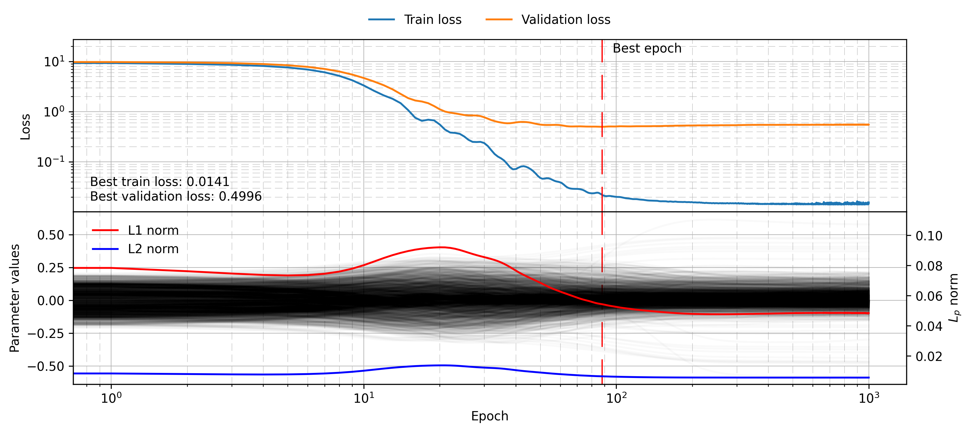
We can see that the L2 and L1 norm do decrease throughout training, and the final validation loss is lower at 0.50, despite the training loss being much larger than before. The regularisation term has indeed improved the model’s generalisation by costing it training performance!
I believe that understanding L2 regularisation is subtle. It isn’t obvious that using smaller weights should prevent the model from naively memorizing the training data or overfitting noise. One potential way of explaining the effect is by considering interpolation and extrapolation. Sometimes fitting a very large degree polynomial to sparse data will work well, hitting every point exactly, but high degree polynomials usually have very pathological behaviour even slightly outside the domain they were trained on. The scikit-learn documentation show a good example of this. Despite this explanation providing a nice visualisation, it isn’t obvious that large weights are in any way analogous to high degree polynomials.
Another way to think of the regularising effect is in terms of statistical learning theory discussed in a previous post, since adding an L2 norm essentially limits the size of the hypothesis class, just in a soft way rather than a hard cutoff. Smaller hypothesis classes can be more easily explored with fewer training samples, which manifests as a lack of overfitting. Considering again the examples of polynomials given above, it is possible to define a series of hypothesis classes \(\mathcal{H}_n\) where the input data is modeled with a maximum power of \(x^n\). This induces an ordering of such classes since \(\mathcal{H}_0 \subset \mathcal{H}_1 \subset \mathcal{H}_2 \cdots\), which can be seen simply by the fact that e.g. linear functions are 2nd degree polynomials with one parameter fixed to zero. Given the chance however, models will not set parameters to zero, and will instead make some use of the higher powers if not penalised for it. This leads to a type of minimisation not based purely on fitting data (empirical risk minimisation, ERM) but instead fitting data while penalising added complexity (structural risk minimisation, SRM). Adding an L2 norm is a soft version of SRM for continuous parameters.
Perhaps the most compelling demonstration of weight decay I have seen comes from chapter 7 of the Deep Learning book, available for free here. By considering a task with approximately quadratic loss function they show mathematically how weight decay forces parameters to be smaller selectively along dimensions with less explanatory power. We will sketch the demonstration here, leaving the full text as a more detailed reference. Firstly, considering the true minimum of the quadratic loss at model parameters \(\boldsymbol{w}\), we can write the loss function as
\[ \mathcal{L}(\boldsymbol{\theta}) = \mathcal{L}(\boldsymbol{w}) + \frac{1}{2} \big( \boldsymbol{\theta}-\boldsymbol{w} \big) \boldsymbol{H} \big( \boldsymbol{\theta}-\boldsymbol{w} \big). \]
Note that this is just the loss function, without any regularisation term added. The Hessian matrix \(\boldsymbol{H}\) evaluated at \(\boldsymbol{w}\) provides the second derivative of the loss function \((\partial^2{\mathcal{L}}/\partial\theta_i\partial\theta_j)\), which here depend on direction in the model parameter space. Seeing this as a Taylor expansion, the first derivative term vanishes since we evaluate at the global minimum, and higher order terms have been dropped. Written in this form, the gradient of the loss term is
\[ \nabla_{\theta_i}\mathcal{L}(\boldsymbol{\theta}) = \sum_j H_{i j}(\theta_j - w_j), \]
which can then be combined with the L2 gradient provided above. Since this is now a matrix problem, we can choose to transform into the eigenbasis of the Hessian matrix, which provides a very nice bottom line solution. For clarity we use greek indices to denote the eigenbasis \(\big(\theta_i\rightarrow\theta_\alpha\big)\). The final regularised model parameters chosen \(\hat{\theta}_\alpha\) are the same as \(w_i\) but rescaled along the eigenvectors given by \(\boldsymbol{H}\). In particular rescaled as
\[ \hat{\theta}_\alpha = w_\alpha\frac{h_\alpha}{h_\alpha+\lambda}, \]
where \(h_\alpha\) is the eigenvalue of \(\boldsymbol{H}\) along eigenvector \(\alpha\). What does this all mean? Directions with a very large eigenvalue are mostly unchanged by the L2 regularisation term. Geometrically this corresponds to seeing no changes in the parameters \(\theta_i\) which affect the loss value significantly. In other words, the effect of L2 regularisation is to shrink the parameter vector only along directions which don’t significantly impact the loss function, therefore preserving most of the neural networks explanatory power on the training set without allowing it to model spurious correlations and noise.
Remark:
There is some subtlety of how to implement weight decay together with optimisers like Adam, as discussed in this fast.ai blog post. Within the training loop provided in the appendix I achieve the same results with the optional optimiser weight decay and manually setting L2 norm in the gradients, which gave me confidence in the implementation of L1 regularisation discussed next.
L1 regularisation
An L1 regularisation term looks deceptively similar to L2, but has very different consequences for training. To be concrete we now add a term \[ \mathcal{L}_{L1}(\boldsymbol{\theta}) = \lambda |\boldsymbol{\theta}| = \lambda \sum_i |\theta_i| \]
to the loss function, containing the absolute value of the parameter vector instead of its squared norm. This means the gradient is now computed by \[ \nabla_{\theta_i}\mathcal{L}_{L1} = \lambda\;\mathrm{sign}(\theta_i), \]
which is a fixed size regardless of the magnitude of the parameter, much different to the L2 case.
Before discussing the effects further let’s visualise them with an experiment:
model = MLP([50, 25, 25, 1])
mlp_l1_reg_histories = training_loop(
    model,
    train_dataset,
    val_dataset,
    num_epochs=2_000,
    lr=0.01,
    l1_reg=0.021,
    device=device
)
plot_training_visualisation(mlp_l1_reg_histories, alpha=0.1)
This time the parameter trajectories reveal a very different story, with many of them collapsing to zero even late into training once the loss is mostly static on the training set. This is why L1 regularisation is often referred to as sparsifying, since it generates sparse statistics (in this case a sparse model parameter vector). Furthermore we can see the regularisation term indeed works, giving a final validation loss of 0.28.
To understand the sparsity, compare the gradients induced by the L1 and L2 regularisation terms. In the latter case we saw that the gradient would shrink in proportion to the parameter itself, meaning the parameter evolution naturally slows as it shrinks, essentially leading to an exponential decay in parameter magnitude to a stable point. In the L1 case there is a constant force opposing each parameter regardless of its size. If we assume a parameter requires some minimal value to provide a positive benefit to the model then L1 regularisation could prevent the parameter from ever reaching a useful state, and therefore it simply collapses to zero. This can manifest as an unstable optimisation, especially early in training. Similarly, late in training if a parameter provides sufficiently small benefit on consecutive batches then it can collapse.
Earlier I advocated for playing with toy problems like these to become more adept with ML, and here we have a great proof of that concept. Recent work by Anthropic uses a sparsifying autoencoder to detect combinations of neurons which correspond to single semantic concepts in large language models. The results are awesome, and I highly recommend readers check it out. Despite the scale of the problem they’re tackling, the principles of sparse autoencoders are evident from a noisy linear regression with 200 training samples. Note that in their case the L1 norm is on activations of neurons, not the weights and biases. This leads to few neurons “lighting up” at once, rather than few weights being non-zero.
Regularisation by minibatch size
Alongside the common explicit norm terms added to the loss function there is also an implicit regularising effect from using small minibatches. Stated another way, the stochasticity within stochastic gradient descent (SGD) itself can promote the model to generalise well. Explaining this rigorously is not simple, but roughly speaking the different possible combinations of training samples the model has to fit itself encourages a model to find more general solutions. In the case of evaluating on the full training set (as we have done so far) the model sees everything at once, and can overfit much easier. A rigorous treatment of this topic can be found in this paper by a team at Google.
Once again the results can be easily seen with direct experimentation:
model = MLP([50, 25, 25, 1])
mlp_minibatch_histories = training_loop(
    model,
    train_dataset,
    val_dataset,
    num_epochs=1_000,
    lr=0.01,
    batch_size=32,
    device=device
)
plot_training_visualisation(mlp_minibatch_histories)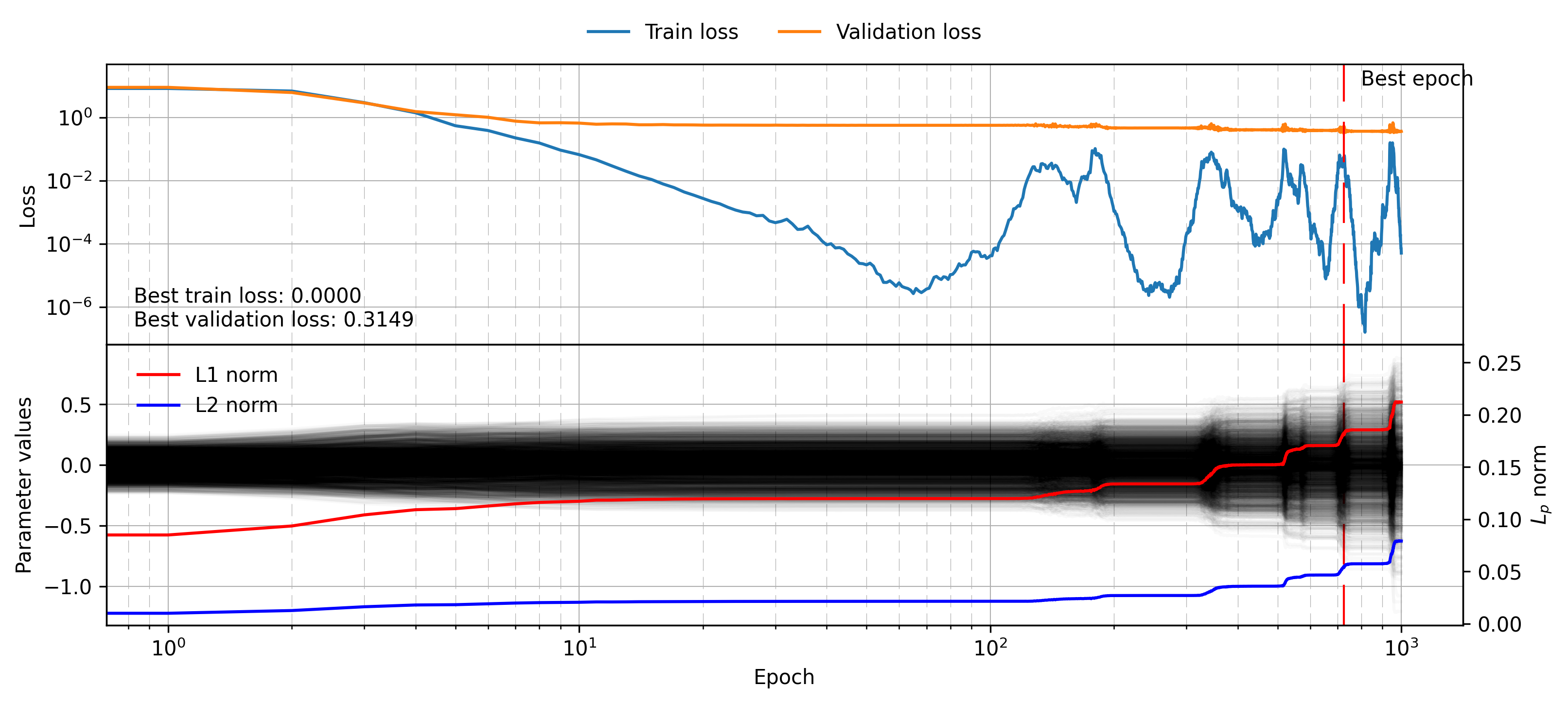
The training dynamics here are admittedly quite unstable. Judging by the loss values hitting very small numbers (\(\sim 10^{-6}\)) I suspect it is due to numerical instabilities creating large gradients which the Adam optimiser takes a while to correct due to the momentum contribution. Despite the strange training loss, it can be seen that the batch size has indeed regularised the results, leading to a validation loss of just 0.31. The parameter vector for this model shows some very interesting behaviour, generally growing over time in a way that matches the aforementioned training instability. Without terms like the L1 and L2 previously discussed there is no incentive for the model to not just grow with time, and I suspect this growing behaviour is actually quite common in real-world problems. This could be why, at least in my experience, many papers employ at least some low weight decay \(\sim 10^{-4}\) , which I suspect stops indefinite growth as well as providing generalisation benefits.
Remark:
This case study provides yet more encouragement that toy models like this can be invaluable to growing ML skills. This insight on growing parameter weights provided me with an idea to solve a problem which is now part of a paper. That project made use of a contrastive loss function which compares different latent space embeddings with cosine similarity, and either enhances or penalises the measured angle subject to some criteria. Within this system there is no implicit penalty at all placed on the overall magnitude of an embedded vector, and it appears that they tended to grow over time, which was bad for downstream results. A small weight decay was sufficient to fix this issue, since by the same logic reducing the magnitude of weights (and therefore the latent space activations) reduced the L2 loss without impacting the contrastive loss negatively.
Dropout
Finally we will consider perhaps the most common regularisation technique alongside weight decay: dropout. This too is initially a strange concept, consisting in setting some activations to zero randomly throughout the forward pass, thus forcing the network to manage a good calculation with some level of redundancy. Let’s see the results of the experiment
model = MLP([50, 25, 25, 1], dropout=0.1)
mlp_dropout_histories = training_loop(
    model,
    train_dataset,
    val_dataset,
    num_epochs=2_000,
    lr=0.01,
    device=device
    )
plot_training_visualisation(mlp_dropout_histories)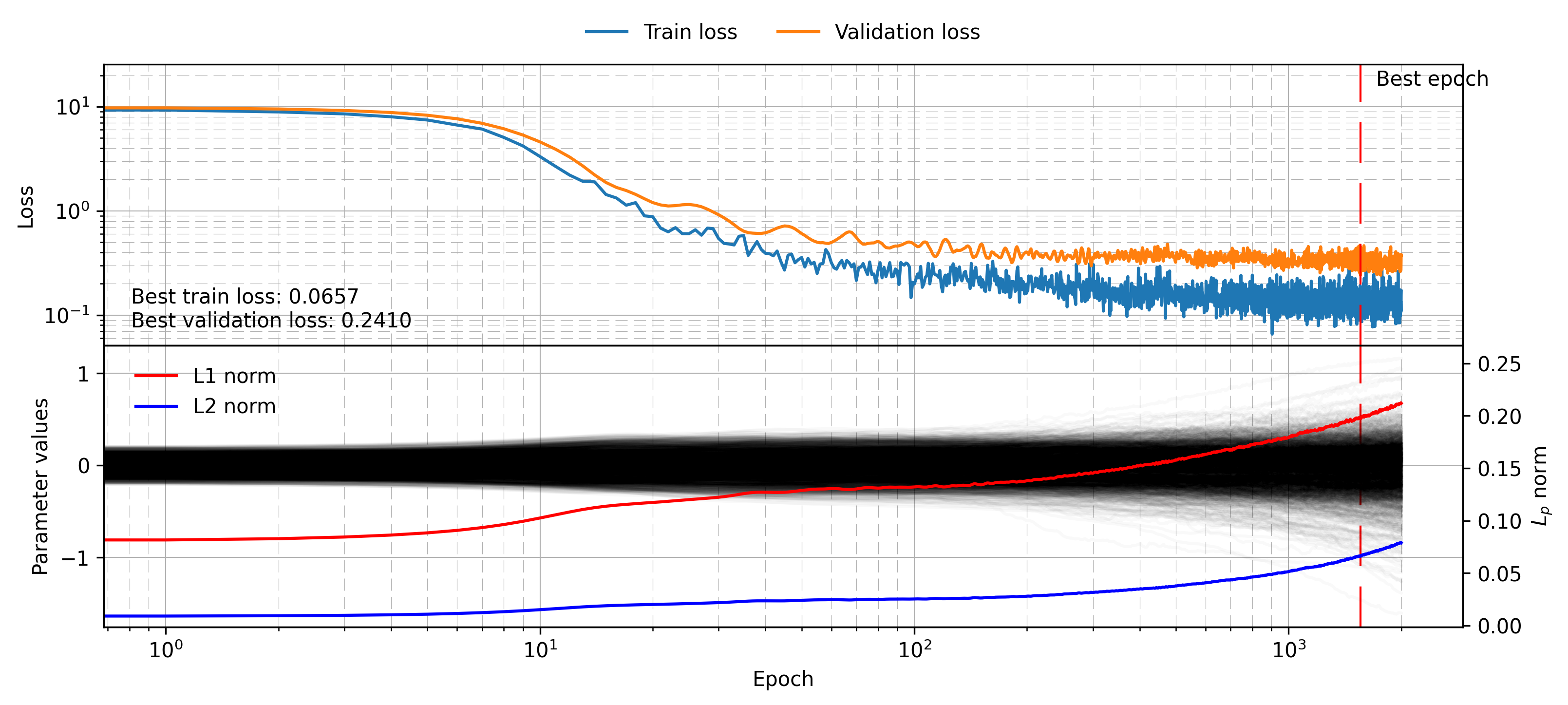
Here again the proof is in the experiment, with the validation loss being much lower at 0.27. Again note the growing parameter weights over time, which could be remedied with a small weight decay. To see why dropout works, first consider training multiple different models on the same task. Each one can overfit, and each one will provide a different flawed estimate of the true labels. If you assume however that the error on each model is uncorrelated, then averaging their results can give an unbiased estimate of true labels. In practice this argument breaks down since the models are not completely uncorrelated, being trained on the same data and possibly with similar architecture or hyperparameters. Still, this very successful concept is the reason we use a random forest and not just a single tree. It is also related to the concept of boosting, which is part of XGBoost, probably one of the most successful out-of-the-box ML algorithms for general tasks.
Returning to dropout, the idea is that by removing neurons at random, there are a vast number of possible subnetworks within a larger network, and each one receives a bit of the training time. The exact number of subnetworks in principle grows as a combinatoric quantity, faster than exponential growth with model size! In practice however there is some parameter tying between each subnetwork, meaning we do not yield gains proportional to training truly independent models. Despite the limitations it is an incredibly cheap and effective way of increasing performance without increasing training cost in a meaningful way.
Comparison
In the following figure we show each model’s performance on a single plot. The linear model sets a benchmark for both training and validation loss, indicated by blue and red dots respectively. In almost every case the MLP models perform better on the training set, but worse on the validation set, a hallmark of overfitting. In more formal language, this is due to the size of the hypothesis class, which in this case is constructed to not improve approximation error, but to still incur the cost of larger estimation error. Upon adding regularisation terms to the MLP model we see the performance gap between training and validation set shrink, but never achieving the performance offered by the linear model. The L1 regularisation and dropout are particularly powerful for this experiment.
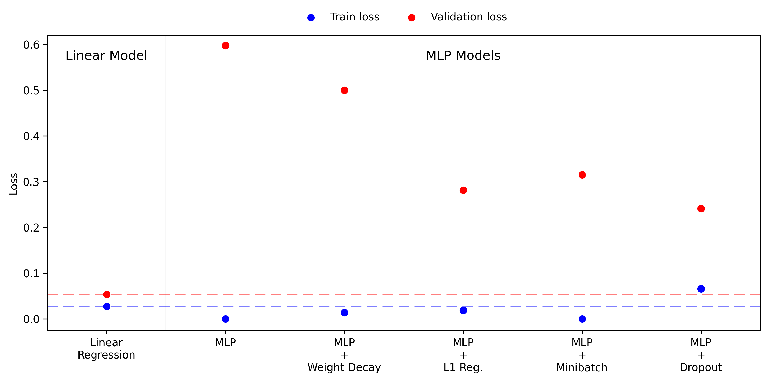
There is one more point I want to add to this story. It is often seen in discussions of model tuning that the first thing you should always do, if possible, is to gather more data. In this context data is the best regulariser, and should always be considered before choosing model size and hyperparameters. Since this is an artificial experiment we can easily generate more data and rerun all the pervious results. The figure below shows the training and validation losses with 400 training points, doubled from the previous 200.
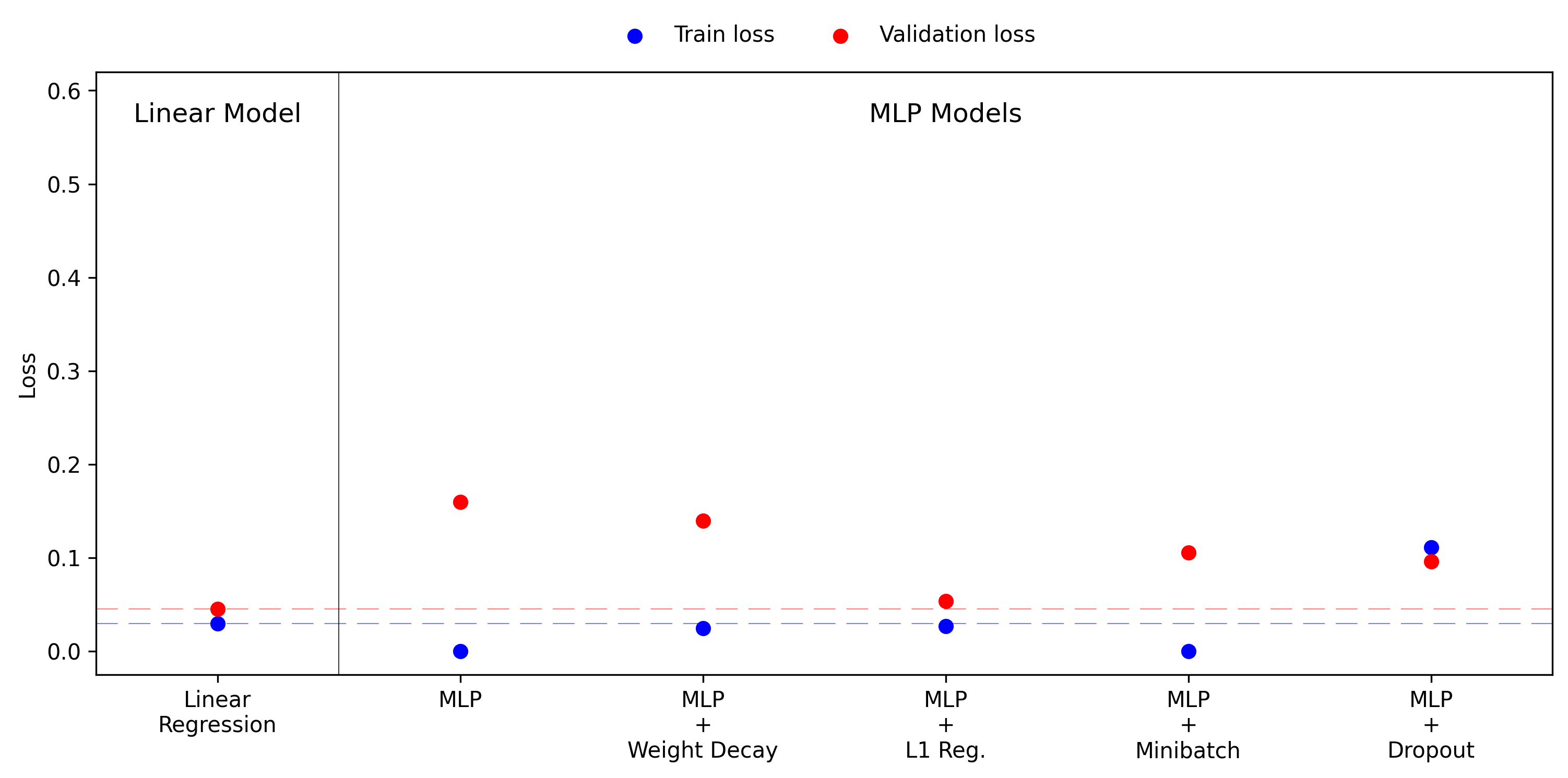
In this case all of the MLP models now perform much better, and even the simplest MLP with 400 training points outperforms all regularised cases with 200 points. Notably, applying L1 regularisation with 400 training points achieves almost optimal performance, as measured by the simple linear model. This illustrates the interplay of data and regularisation, they can work together to derive strong results, but regularisation on its own can only go so far.
Conclusion
I wanted to write this blog to explore regularisation quantitatively after reading the perspective of Ian Goodfellow, Yoshua Bengio and Aaron Courville in their Deep Learning book. I was surprised that in their eyes regularisation was far more than a useful trick, and actually central to the entire premise of deep learning. Combining this with my previous reading of statistical learning theory I think I can understand why. Deep learning proposes constructing vast hypothesis class, capable of modeling almost any desirable function. This comes at a very large cost, since searching through these spaces requires a lot of data. Regularisation techniques offer data agnostic approaches to making this function space search more efficient and more effective. Without these techniques deep learning would be almost guaranteed to fail in all but the most data intense domains. This concept is illustrated, somewhat metaphorically, in the thumbnail to this post: we should try to keep our hypothesis class appropriately boxed in, yielding the power from deep hierarchical models without the enormous penalty of too many neurons.
Appendix (Code snippets)
Code available at github.com/TomKite57/regularisation_blog.
Data generation
import torch

reset_seeds()

train_size = 200
val_size = 10_000
noise_coeff = 0.2
dims = 50
true_weights = torch.randn(dims, 1)*3/np.sqrt(dims)
true_intercept = torch.randn(1)

with torch.no_grad():
    train_sample_x = torch.randn(train_size, dims)
    train_sample_y = train_sample_x @ true_weights + true_intercept + torch.randn(train_size, 1)*noise_coeff

    val_sample_x = torch.randn(val_size, dims)
    val_sample_y = val_sample_x @ true_weights + true_intercept + torch.randn(val_size, 1)*noise_coeff

    train_dataset = torch.utils.data.TensorDataset(train_sample_x, train_sample_y)
    val_dataset = torch.utils.data.TensorDataset(val_sample_x, val_sample_y)
Training loop
import torch
from collections import defaultdict
from tqdm.notebook import tqdm as tqdm_nb
import numpy as np

def training_loop(model,
                  train_dataset, validation_dataset,
                  weight_decay=0, l2_reg=0, l1_reg=0,
                  batch_size=None, lr=0.01, num_epochs=2_500,
                  criterion=torch.nn.MSELoss(),
                  device=None,
                  optimiser="adam"):

    # Set seed for reproducibility
    reset_seeds()

    if device is None:
        device = "cpu"
    model.to(device)

    # Record training history
    histories = defaultdict(list)

    # Set up batch sizes and loader
    batch_size = min(batch_size, len(train_dataset)) \
        if batch_size else len(train_dataset)
    train_loader = torch.utils.data.DataLoader(train_dataset,
        batch_size=batch_size, shuffle=True, drop_last=True)
    validation_loader = torch.utils.data.DataLoader(validation_dataset,
        batch_size=len(validation_dataset), shuffle=False, drop_last=True)

    # Set up optimiser and loss function
    if optimiser == "adam":
        optimiser = torch.optim.Adam(model.parameters(),
        lr=lr, weight_decay=weight_decay)
    elif optimiser == "adamw":
        optimiser = torch.optim.AdamW(model.parameters(),
        lr=lr, weight_decay=weight_decay)
    elif optimiser == "sgd":
        optimiser = torch.optim.SGD(model.parameters(),
        lr=lr, weight_decay=weight_decay)
    else:
        raise ValueError("Optimiser not recognised.")
    criterion = criterion.to(device)

    # Record best epoch
    best_model_state = None
    best_loss = np.inf

    # Starting point
    with torch.no_grad():
        histories["model_state"].append(model.get_weights())
        train_loss = []
        for x, y in train_loader:
            x, y = x.to(device), y.to(device)
            train_loss.append(criterion(model(x), y).item())
        histories["train_loss"].append(np.mean(train_loss))
        val_loss = []
        for x, y in validation_loader:
            x, y = x.to(device), y.to(device)
            val_loss.append(criterion(model(x), y).item())
        histories["val_loss"].append(np.mean(val_loss))

    # Training loop
    for epoch in tqdm_nb(range(num_epochs)):
        model.train()
        epoch_losses = []
        for x, y in train_loader:
            x, y = x.to(device), y.to(device)
            optimiser.zero_grad()
            y_pred = model(x)
            loss = criterion(y_pred, y)
            loss.backward()

            # Manual regularisation
            if l2_reg:
                for param in model.parameters():
                    if param.requires_grad:
                        param.grad.data += l2_reg*param.data
            if l1_reg:
                for param in model.parameters():
                    if param.requires_grad:
                        param.grad.data += l1_reg*torch.sign(param.data)

            optimiser.step()
            epoch_losses.append(loss.item())

        # Record batch
        histories["train_loss"].append(np.mean(epoch_losses))
        histories["model_state"].append(model.get_weights())

        # Record validation loss
        model.eval()
        epoch_losses = []
        with torch.no_grad():
            for x, y in validation_loader:
                x, y = x.to(device), y.to(device)
                val_loss = criterion(model(x), y)
                epoch_losses.append(val_loss.item())

        histories["val_loss"].append(np.mean(epoch_losses))

        if histories["val_loss"][-1] < best_loss:
            best_loss = histories["val_loss"][-1]
            best_model_state = model.state_dict()

    # Convert to numpy arrays
    for key, value in histories.items():
        histories[key] = np.array(value)

    # Load best model
    model.load_state_dict(best_model_state)
    model.to("cpu")
    histories["model"] = model

    return histories
Training visualisation plot
import matplotlib.pyplot as plt
import numpy as np

def plot_training_visualisation(histories, l1_line=True, l2_line=True, alpha=0.025, savename=None):
    fig, [ax1, ax2] = plt.subplots(2, 1, figsize=(12, 5), sharex=True, dpi=100)
    plt.subplots_adjust(hspace=0, wspace=0)

    ax1.plot(histories["train_loss"], label="Train loss")
    ax1.plot(histories["val_loss"], label="Validation loss")
    best_epoch_str = "\n".join([
        f"Best train loss: {np.min(histories['train_loss']):.4f}",
        f"Best validation loss: {np.min(histories['val_loss']):.4f}"
    ])
    ax1.text(0.02, 0.05, best_epoch_str,
        ha='left', va='bottom', transform=ax1.transAxes)
    best_epoch = np.argmin(histories["val_loss"])
    ax1.axvline(best_epoch, color='r', dashes=[20,10], lw=1)
    ax2.axvline(best_epoch, color='r', dashes=[20,10], lw=1)
    ax1.text(best_epoch*1.1, 0.95, f"Best epoch",
        va='top', ha='left', transform=ax1.get_xaxis_transform())
    ax1.set(xlabel="Epoch", ylabel="Loss", yscale="log", xscale="log")
    ax1.grid(which='major', linestyle='-', linewidth=0.5)
    ax1.grid(which='minor', dashes=[20,10], linewidth=0.3)
    ax1.legend(loc="lower center", bbox_to_anchor=(0.5, 1.01), ncol=2, frameon=False)

    num_params = histories["model_state"].shape[1]
    for i in range(num_params):
        l = ax2.plot(histories["model_state"][:, i], alpha=alpha, color='k')
    if l1_line or l2_line:
        twin_ax2 = ax2.twinx()
    if l1_line:
        twin_ax2.plot(np.sum(np.abs(histories["model_state"]), axis=1), label="L1 norm", color='r')
    if l2_line:
        twin_ax2.plot(np.sum(np.square(histories["model_state"]), axis=1), label="L2 norm", color='b')

    ax2.set(xlabel="Epoch", ylabel="Parameter values", yscale="linear", xscale="log")
    ax2.grid(which='major', linestyle='-', linewidth=0.5)
    ax2.grid(which='minor', dashes=[20,10], linewidth=0.3)
    if l1_line or l2_line:
        twin_ax2.legend(loc="upper left", bbox_to_anchor=(0.01, 0.99), ncol=1, frameon=False)
        twin_ax2.set(ylabel="$L_p$ norm")

    if savename:
        plt.savefig(f"figures/{savename}", dpi=300, bbox_inches='tight')
    plt.show()
Final comparison plot
model_names = [
    "Linear\nRegression",
    "MLP",
    "MLP\n+\nWeight Decay",
    "MLP\n+\nL1 Reg.",
    "MLP\n+\nMinibatch",
    "MLP\n+\nDropout",
]
histories = [
    linear_regression_histories,
    mlp_histories,
    mlp_weight_decay_histories,
    mlp_l2_reg_histories,
    mlp_l1_reg_histories,
    mlp_minibatch_histories,
    mlp_dropout_histories,
]

fig, ax = plt.subplots(1, 1, figsize=(12, 5))
for ind, (name, history) in enumerate(zip(model_names, histories)):
    best_train_loss = min(history['train_loss'])
    best_val_loss = min(history['val_loss'])
    ax.scatter(ind, best_train_loss, c='b', label='Train loss' if ind == 0 else None)
    ax.scatter(ind, best_val_loss, c='r', label='Validation loss' if ind == 0 else None)

    if ind == 0:
        ax.axhline(best_train_loss, c='b', dashes=[20,10], alpha=0.5, lw=0.5)
        ax.axhline(best_val_loss, c='r', dashes=[20,10], alpha=0.5, lw=0.5)

ax.axvline(0.5, c='k', ls='-', alpha=0.75, lw=0.5)
ax.text(0, 0.95, 'Linear Model', ha='center', va='top', fontsize=12, transform=ax.get_xaxis_transform(), c='k')
ax.text(3, 0.95, 'MLP Models', ha='center', va='top', fontsize=12, transform=ax.get_xaxis_transform(), c='k')

ax.set_xticks(range(len(model_names)))
ax.set_xticklabels(model_names, rotation=0)
ax.set(ylabel='Loss', ylim=(-0.025, 0.62), xlim=(-0.5, len(model_names)-0.5))
ax.legend(loc='lower center', bbox_to_anchor=(0.5, 1.01), ncol=2, frameon=False)
plt.savefig("figures/benchmark_results.png", dpi=300, bbox_inches='tight')
plt.show()