Exploring the Mathematics of Statistical Learning Theory

Exploring the Mathematics of Statistical Learning Theory

It is impossible to deny the power of neural networks – recent progress in deep learning has consolidated them as the approach of choice for many learning tasks. There is, however, still a delicate art to their design, application and training. This post will dig into statistical learning theory, which provides some theoretical backbone to the fundamental tradeoffs present in any learning task, which in turn illuminates some of the nuances present in the current machine learning landscape.

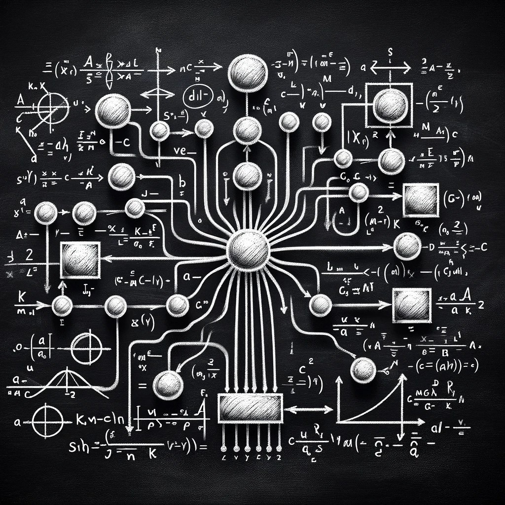A depiction of the connection between machine learning and mathematics. Generated by DALL·E 3

Introduction

A neural network (NN) with an infinite single dense hidden layer can approximate any function. When I first learned about the universal approximation theorem I was in awe. I knew NNs were powerful in practice, but learning they can do anything in principle felt huge – I thought perhaps we really can capture intelligence this way. Of course there is always a tradeoff, and a common discussion that follow that of universal approximation is the argument that the data needed to train a network grows incredibly fast with its size, not to mention the computing power. In fact, it is argued that the data needed to train a model grows exponentially with its size.

In this post I want to introduce various notions from statistical learning theory which quantify some of the considerations mentioned above. This post will be more mathematical and theoretical in nature, but I have honestly found myself thinking differently about my own uses of machine learning since breaching this challenging topic. I hope others will find it similarly useful and interesting.

The main source for this post is Understanding Machine Learning: From Theory to Algorithms. A lot of this text will follow their notation and choice of topics. However I am also borrowing some of the philosophy from the Geometric Deep Learning project. Finally, a popular set of notes which discuss these notions can be found in the CS229 lectures.

What are we learning, and how?

As many mathematics courses tend to do, we will start with numerous definitions to have a common language to build on. The basic idea of learning is to predict some features $y$ from some set of input variables $x$. Oftentimes we will have $\underset{―}{\mathbf{x}}$ and $\underset{―}{\mathbf{y}}$, where boldface and underlined symbols are vectors, which in this context can simply be thought of as a package for many variables. As a common example, perhaps we’re predicting both the cost of a house and typical time for sale from the country, floor size and number of bathrooms: $$\begin{array}{cc}\underset{―}{\mathbf{y}}=\left(\begin{array}{c}{y}_{\text{cost}},\\ y_{\text{time}}\end{array}\right)& \underset{―}{\mathbf{x}}=\left(\begin{array}{c}{x}_{\text{country}}\\ x_{\text{size}}\\ x_{\text{bathrooms}}\end{array}\right)\end{array}.$$

In the context of supervised learning we learn to make predictions by observing samples of paired inputs and outputs, and using these to build a predictive function $f(x)\approx y$. This set of examples is commonly known as the training set $S=\{(x_1,y_1),...,(x_m,y_m)\}$. Building a function this way is known as Empirical Risk Minimization (ERM).

The notation so far will serve us well, but we can get a little more abstract still (and use fancy fonts in the process). The space of all possible inputs is $\mathcal{X}$, so concretely $x\in \mathcal{X}$. Similarly for the labels $y\in \mathcal{Y}$, where often we will have $\mathcal{Y}=\{1,0\}$ as in classification tasks. Each possible pairing of input and output is then an element of $\mathcal{X}\times \mathcal{Y}$. Considering the joint input feature and label space is important, as it allows us to consider cases where the same input sometimes has different labels, meaning that we have a distribution over the joint space with no strict function from $\mathcal{X}$ to $\mathcal{Y}$ (see remark below). A final concept linking all this together is to have a probability distribution $\mathcal{D}$ over the space $\mathcal{X}\times \mathcal{Y}$, allowing for some inputs/labels to be more common than others, an important considering when evaluating the performance of the learned function (mistaking rare inputs is less bad than mistaking the typical ones).

To give an example of when the probability distribution approach is helpful in making the mathematics concrete, consider a loss function $\ell (f(x),y)\ge 0$ which compares the output of a function $f$ on the input $x$ to the known answer $y$. This loss function (or sometimes called risk) is often squared loss $\ell (a,b)=(a-b{)}^2$ or 0-1 loss in the case of classification $\ell ={\mathbb{1}}_{a\ne b}$. The loss between pairs of labels induces a measure of loss on the function itself, defined as the expectation value of the loss over the distribution of $\mathcal{X}\times \mathcal{Y}$:

$$L_{\mathcal{D}}(f)=\underset{(x,y)\sim \mathcal{D}}{\mathbb{E}}\ell (f(x),y).$$

Similarly we can define the loss over the training sample (or any other subset of $\mathcal{X}\times \mathcal{Y}$) as $L_S(f)$:

$$L_S(f)=\frac{1}{m}\sum _{i=1}^m\ell (f(x_i),y_i).$$

By the law of large numbers we can say that $L_S(f)\approx L_{\mathcal{D}}(f)$ for large $m$. This makes the ERM approach legitimate, but as we will see below, the question of how large is large enough for $m$ is the key question.

Remark:

One key assumption we can make is that the target function we want to learn does indeed exist $f^{\ast }(x)=y$, and the goal then is to find it or approximate it with some other function $f(x)\approx f^{\ast }(x)$. This is known as the realizability assumption, and is equivalent to stating that there exists $f^{\ast }$ such that $L_{\mathcal{D}}(f^{\ast })=0$. This also implies that $L_S(f^{\ast })=0$ for that same function, while the contrary is not true for all functions. In practice the realizability assumption is not necessary and is often not at all realistic. Consider for example a character level language model as often considered by Andrej Karpathy, where the following character is predicted based on the previous $n$ characters. Taking the case $n=3$ this means allowing $\mathtt{G}\mathtt{R}\mathtt{A}$ to become any of $\{\mathtt{G}\mathtt{R}\mathtt{A}\mathtt{B},\mathtt{G}\mathtt{R}\mathtt{A}\mathtt{D},\mathtt{G}\mathtt{R}\mathtt{A}\mathtt{M},\mathtt{G}\mathtt{R}\mathtt{A}\mathtt{N},\mathtt{G}\mathtt{R}\mathtt{A}\mathtt{Y}\}$. This is not a valid function in the usual mathematical sense since a single input $x$ maps to various possible outputs. The best we can hope to do is predict a distribution of possible letters (with associated probabilities). In practice this means that there would be a minimal value of the loss function which is always non-zero. Once this non-zero minimal loss is included, many proofs within statistical learning theory remain essentially the same.

Coming from a physics background the way I like to interpret the lack of realizability is through marginal distributions. Taking the example of house prices, we could imagine that if you had access to hundreds or thousands of other important variables then it would be possible to give an exact price for the house (property energy rating, space for parking, windows facing east or west, etc…). This could be a much larger input space $\overline{\mathcal{X}}\times \mathcal{Y}$ which we do not have access to. When some variables are not known or observable, we achieve the smaller distribution by adding up the possibilities, or integrating over them. The logic is that many inputs $(\overline{x},y)\in \overline{\mathcal{X}}\times \mathcal{Y}$ in the larger space will all be recognized as the same input $(x,y)\in \mathcal{X}\times \mathcal{Y}$ in the smaller space, so we add all label possibilities. Mathematically we could write

$${\mathcal{D}}_{\mathcal{X}\times \mathcal{Y}}=\int {\mathcal{D}}_{\overline{\mathcal{X}}\times \mathcal{Y}}\mathrm{d}{\tilde{x}}_i,$$

where $\tilde{x}$ denotes a variable that is unseen in the smaller distribution. This type of randomness in label $y$ for the same $x$ is sometimes called epistemic randomness, since it is based on our lack of knowledge. An alternative is that some things just truly are random, which is known as aleatory randomness. I believe that the distinction between these two matters more in principle than in practice, although I favor the former over the latter.

Simple Example

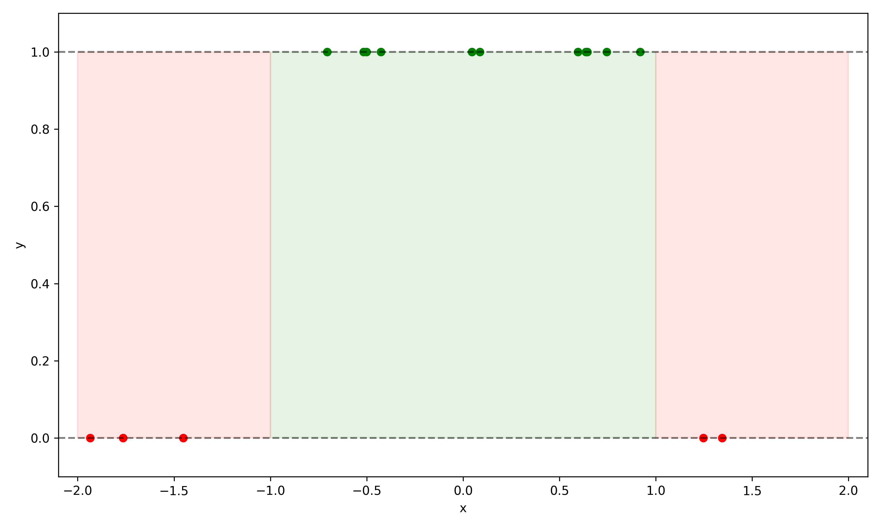
Let’s illustrate an example. We will consider a toy system with a single valued input $x$ evenly distributed in the domain $x\in (-2,2)$, and all values $x\in (-1,1)$ have $y=1$, and $y=0$ otherwise:

$$y=\{\begin{array}{ll}1& \text{if }-1<x<1\\ 0& \text{otherwise}\end{array}$$

This is illustrated in the figure below, with a training set of 16 points scattered.

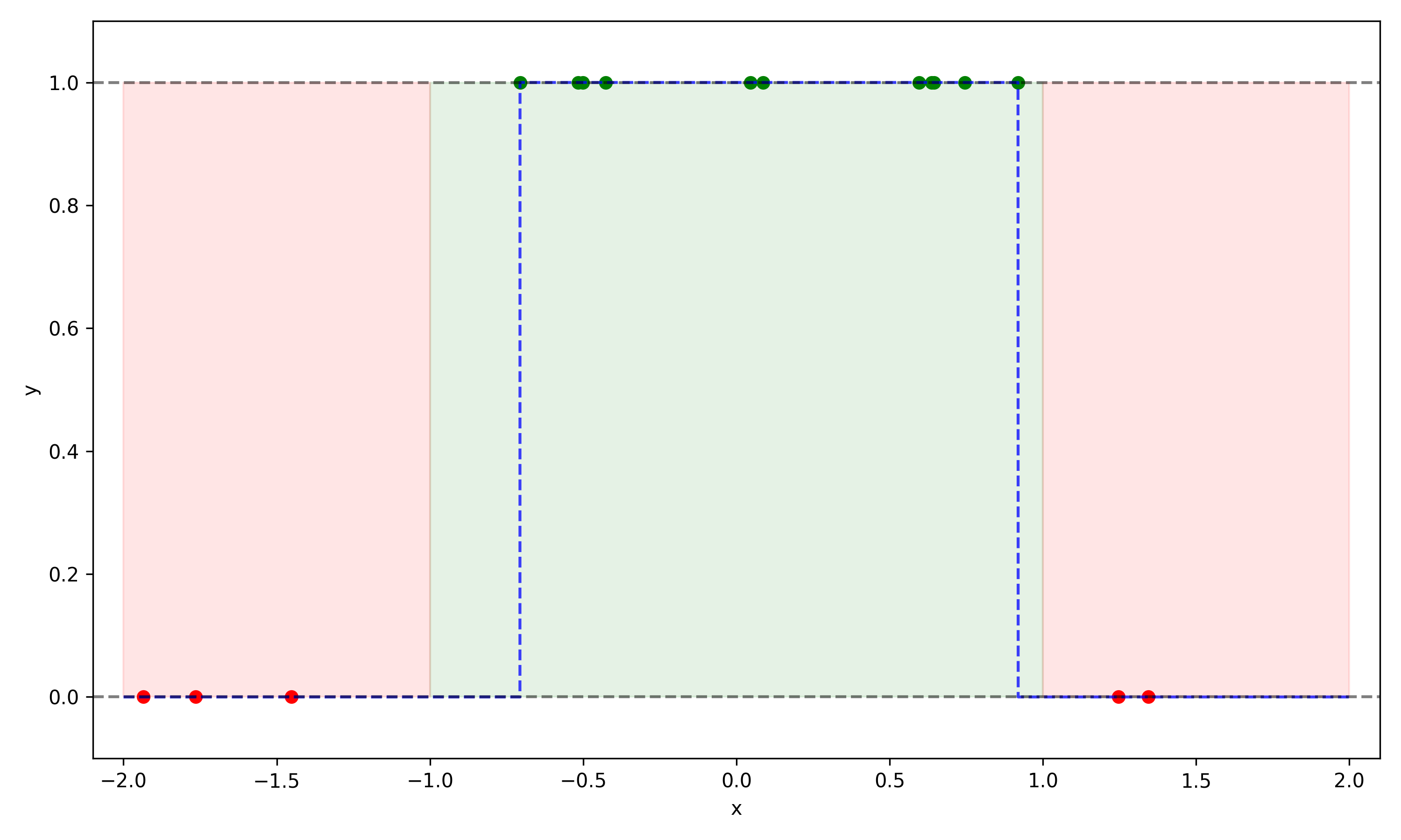
The approach we will take to learning these samples is to build an auxiliary function $g(x)$ such that our learned function $f(x)$ follows

$$f(x)=\{\begin{array}{ll}1& \text{if }g(x)\ge 1\\ 0& \text{otherwise}\end{array}.$$

Below is an example of such a $g(x)$ which performs perfectly on the training data, and would perform reasonably well on new examples:

Below we show a second example which much less natural, and more complicated than the first:

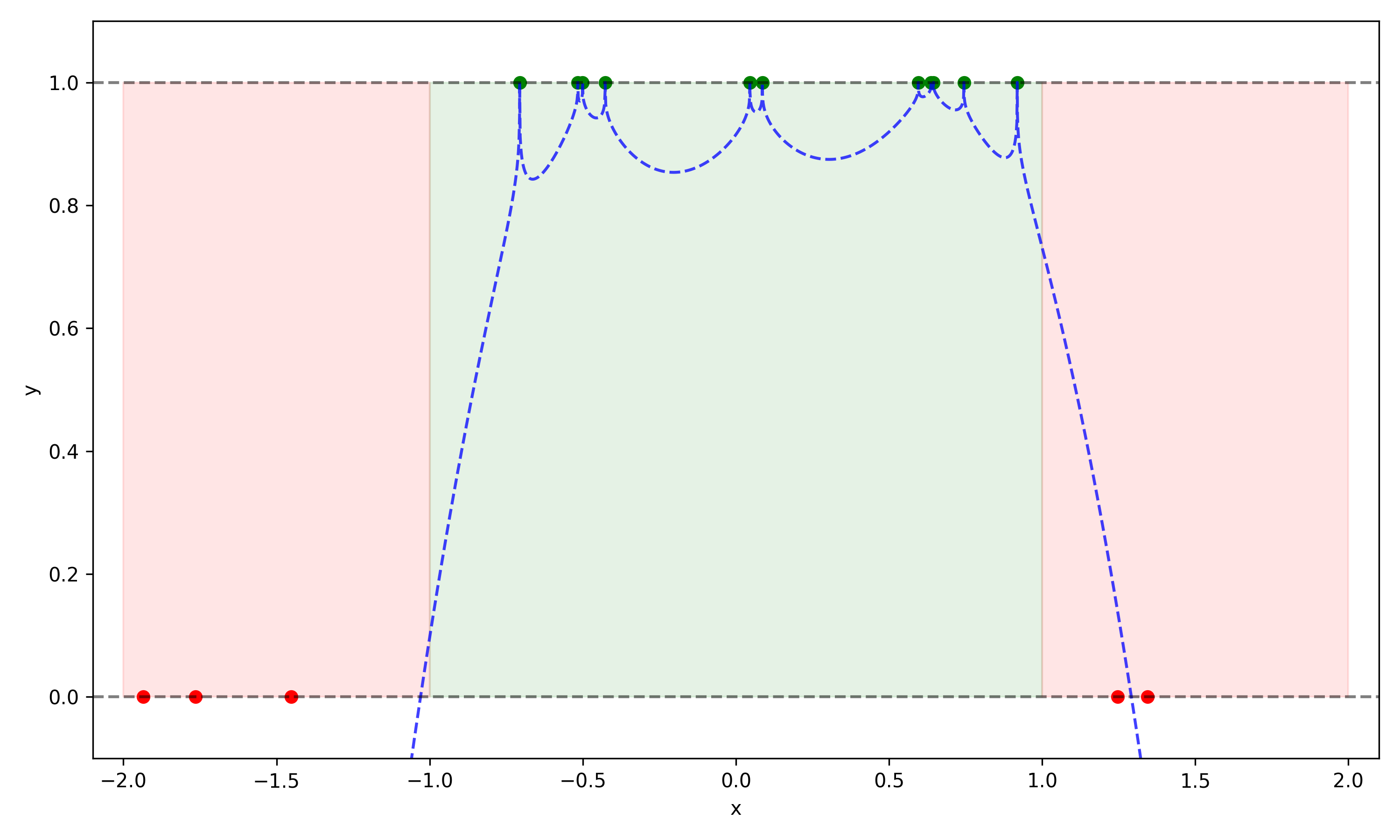
Clearly the second function $g(x)$, while perfectly capturing the training set, will have very poor performance on any new samples. In particular it will have many false negatives. This lesson to be learned here is that choosing an arbitrarily complex function is not a good approach, since its ability to extrapolate is in no way guaranteed.

This particular example was an example of Occam’s razor: the simpler hypothesis was preferable, and extrapolated better to new samples. However if we constructed a new example with two separated green regions, then we would have needed a bit more complexity than the first function offered. The conclusion here is that we want to build learned functions which are as simple as possible, but no simpler.

As a second point, note that this system is realizable, since each $x$ has a unique $y$. It is also realizable within our choice of function, however if we had two disconnected regions with $y=1$ then our choice would have been incapable of realizing a perfect solution.

Inductive Bias

We have seen that using arbitrarily complicated functions to model the training data is not a good approach. However, due to the artificially simple example above, the $g(x)$ that did perform well was constructed with striking resemblance to the true distribution of the data. With real world problems we are hard pushed to pick a learned function that is so well suited to the problem. The ability to pick a good set of functions to learn from depends on our prior beliefs about the system we are studying.

We can formalize this idea: we aim to select the best performing function $f$ from a set of many functions called a hypothesis class $\mathcal{H}$, defined as a set containing mappings from input space to label space $h:\mathcal{X}\to \mathcal{Y}$. Choosing a hypothesis class is one way of encoding prior knowledge of the system.

For example, if we had a single input and a single output a valid hypothesis class would be all linear functions $$\mathcal{H}=\{f_{m,c}(x)=mx+c|m,c\in \mathbb{R}\}.$$

Another valid class would be the set of quadratic polynomials. Or a third set could be the union of those two, although in practice the quadratic choices would almost always have lower loss than the linear functions, making this construction not very helpful. Alternatives to ERM tackle this issue (see Structural Risk Minimization).

Hypothesis classes can also be much more complicated, like a NN governed by millions of parameters instead of two. It could also be something more geometric, like choosing a hyperrectangle in the $\underset{―}{\mathbf{x}}$ space where all labels within the hyperrectangle are $1$, and all other values are $0$. It could also be a set of all decision trees with a maximum depth. The possibilities are vast, and the choice of hypothesis class comes with large tradeoffs to consider.

Bias-Complexity Tradeoff

The main tradeoff under consideration in statistical learning theory is known as the bias-complexity tradeoff, or bias-variance tradeoff. This tradeoff is strongly connected to under and overfitting, which is an important topic in the modern landscape of deep learning (see also double descent). I see there being multiple ways of heuristically describing this tradeoff, one of them being that a large hypothesis class has an extremely strong ability to memorize spurious correlations in the finite training set. Sometimes it is common to hear that the model starts to memorize noise instead of signal, but it is important to remember this phenomenon exists independent of noisy data.

I personally think the idea of memorizing data rather than learning data is appropriate. Consider the example given above where the more complicated second function memorized all previously seen training data, but learned nothing about the true underlying distribution of the data. Even if the model isn’t capable of memorizing all previous seen data, it could be memorizing spurious correlations.

Remark:

A second tradeoff, less important in the context of learning theory, is that searching for the best performing function in a hypothesis class can be computationally expensive, and infeasible in practice. Sometimes, like in the case of a straight line, we can solve the problem analytically. In other cases, like with NNs, we can use backpropagation to quickly optimize millions or billions of parameters to find a well performing function, but even then there is a level of randomness, and running the same code many times will yield different results. In general we can argue that the problem risks becoming combinatorially expensive. For example, imagine a hypothesis class governed by selecting $N$ binary $0/1$ choices (maybe something akin to a decision tree), the total number of function choices is then $2^N$. We can emphasize this point by noting that even $N=266$ would be larger than ${10}^{80}$, the commonly used estimate for the number of fundamental particles in the observable universe.

Sources of Error

Using the notation introduced above we have that the mean loss of a hypothesis $h$ over the entire distribution is denoted as $L_{\mathcal{D}}(h)$. The training loss over our training set $S$ is denoted as $L_S(h)$. The optimal hypothesis, denoted as $h_{\ast }$, is the one that minimizes the loss over the entire distribution,

$$h_{\ast }=\underset{h\in \mathcal{H}}{\mathrm{a}\mathrm{r}\mathrm{g}\mathrm{m}\mathrm{i}\mathrm{n}}{L}_{\mathcal{D}}(h).$$

However, in practice, we do not have access to the underlying distribution, making $h_{\ast }$ inaccessible to us. Instead, we derive our hypothesis from the training set, denoted as $h_S$, which minimizes the training loss,

$$h_S=\underset{h\in \mathcal{H}}{\mathrm{a}\mathrm{r}\mathrm{g}\mathrm{m}\mathrm{i}\mathrm{n}}{L}_S(h).$$

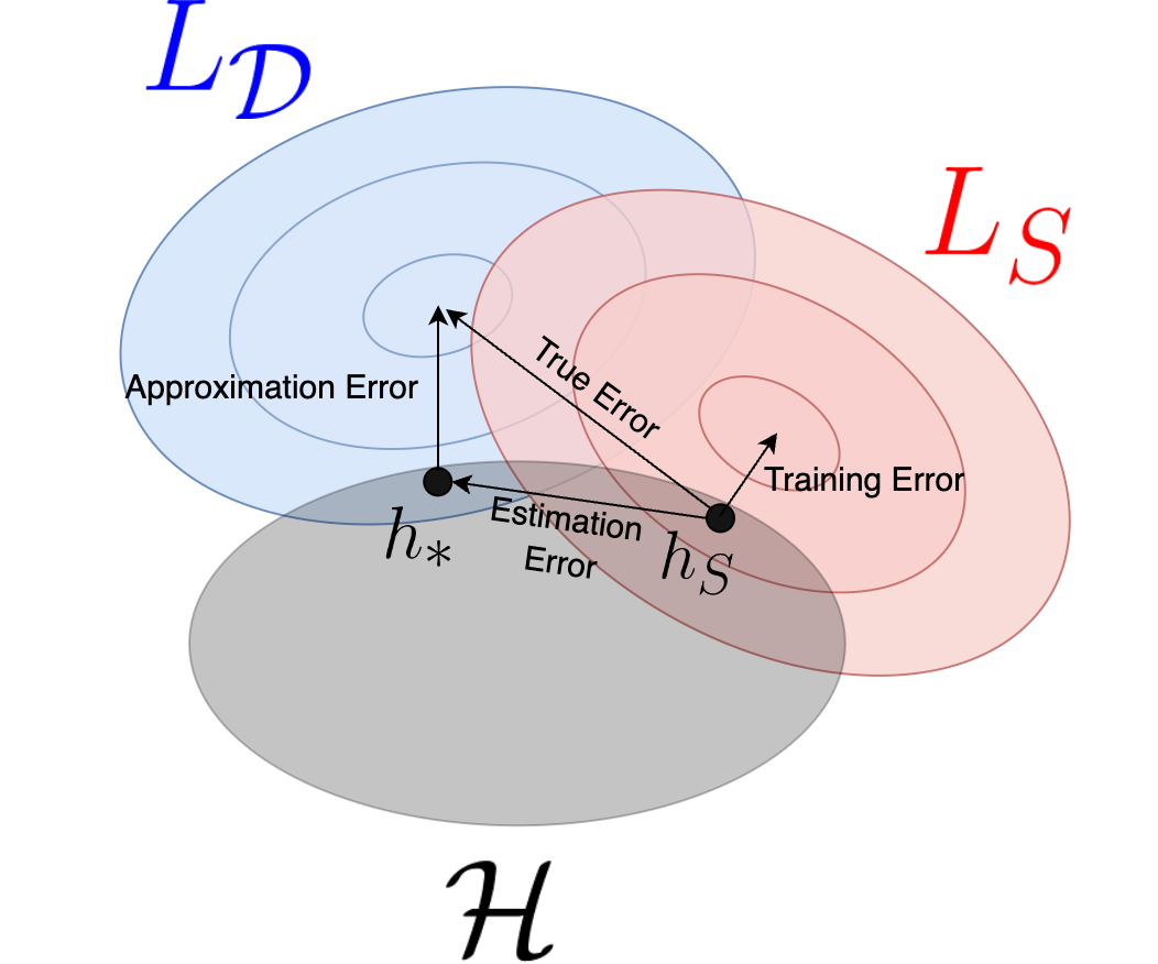
Two distinct sources of error are already present here. Firstly our hypothesis class might be too limited to fit the problem perfectly. We quantify this as the approximation error: $E_{\mathrm{a}\mathrm{p}\mathrm{p}\mathrm{r}\mathrm{o}\mathrm{x}}=L_{\mathcal{D}}(h_{\ast })$. Note that if we do not assume realizability then this would be measured relative to an optimal predictor with nonzero loss. A second source of error is due to estimating the function from a training set rather than the whole distribution, which prevents us finding the optimal function, and is thus called the estimation error or generalisation error, $E_{\mathrm{e}\mathrm{s}\mathrm{t}\mathrm{i}\mathrm{m}\mathrm{a}\mathrm{t}\mathrm{e}}=L_{\mathcal{D}}(h_S)-L_{\mathcal{D}}(h_{\ast })$. These definitions allow us to express the true error $L_{\mathcal{D}}(h_S)$ (again, inaccessible to us) as the sum of the approximation error and the estimation error.

$$\begin{array}{rl}{L}_{\mathcal{D}}(h_S)& =E_{\mathrm{e}\mathrm{s}\mathrm{t}\mathrm{i}\mathrm{m}\mathrm{a}\mathrm{t}\mathrm{e}}+E_{\mathrm{a}\mathrm{p}\mathrm{p}\mathrm{r}\mathrm{o}\mathrm{x}}\\ & =(L_{\mathcal{D}}(h_S)-L_{\mathcal{D}}(h_{\ast }))+L_{\mathcal{D}}(h_{\ast }).\end{array}$$

In the equation above the cancellation is trivial to see mathematically (it is essentially $a=a-b+b$), but something interesting has happened conceptually. We have decomposed the loss into two terms, one of which we expect to decrease with more samples, and one that will only decrease with a new hypothesis class. This relationship is depicted in the following diagram, where we represent hypotheses in some hypothetical 2D plane. Our limited hypothesis class does not allow us to achieve the lowest possible $L_{\mathcal{D}}$ (i.e. we’re depicting that some other function not in $\mathcal{H}$ performs better). If we had more training samples then the $L_S$ contours would approach the true $L_{\mathcal{D}}$ contours, and $h_s$ would therefore approach $h_{\ast }$.

A diagram showing different errors upon selecting a hypothesis. Inspired by a similar diagram shown in the GDL lecture series

With these errors defined we can clarify the bias-complexity tradeoff. Generally speaking, by increasing our number of training samples we can reduce the estimation error. However, if our hypothesis class is chosen poorly, then there will be an irreducible approximation error. Suppose then we want to build a bigger hypothesis class to reduce the approximation error. This leads to each training sample being less informative, and the estimation error will be larger – searching in a larger space requires more data. This is the tradeoff at the heart of statistical learning theory, and much of machine learning practice. It is crucial to build a small hypothesis class which still somehow manages to model the true nature of the system being learned.

In the previous paragraph I used the word “generally”. Can we be confident that decreasing estimation error is really just a case of having more samples? It turns out that it is not always the case, as even our simple example above proves. Loosely speaking, because of the infinite numbers in the range $(-1,+1)$ we would need correspondingly infinite samples to ever have guarantees on the second $g(x)$ we constructed.

In the following section we will make these two distinct cases much more quantitative.

Fundamental Theorem of Learning

We can now introduce the precise mathematical notion of learnability. The way it works is by providing probabilistic guarantees on the error of a learned hypothesis.

As a prelude it is worth recapping the way continuity and calculus is studied in a rigorous mathematical sense. While in practice we’re comfortable in simply taking derivatives and running calculations, the mathematics which underpins the operations of differentiation is based on an interplay between small limits $ϵ$ and $\delta$ and having certain guarantees. Concretely a function $f$ which is continuous at a point $x_0$ can guarantee that a when studying a small deviation $ϵ$ from its image $f(x)\in (f(x_0)-ϵ,f(x_0)+ϵ)$, there exists a small deviation $\delta$ from that point such that all arguments $x\in (x_0-\delta ,x_0+\delta )$ have images in $ϵ$ range. Simply stated (for a 1D example), you draw an $ϵ$ bound on the y-axis and I am guaranteed to have a $\delta$ bound on the x-axis satisfying it.

The concept of learnability follows a similar pattern. In this case you must guarantee that there is only a small probability $\le \delta$ of having an estimation error $\ge ϵ$ upon training on $m$ samples. More importantly, for all possible values of $\delta$ and $ϵ$ you can provide an upper bound on the samples needed, some function $m(\delta ,ϵ)$. This notion of learnability in particular is called Probably Approximately Correct (PAC), where the “probably” is due to $\delta$, and “approximately” is due to $ϵ$.

Using symbols, in a PAC learnable hypothesis class $\mathcal{H}$ we have that with probability of at least $1-\delta$, upon training on $m\ge m(\delta ,ϵ)$ samples:

$$L_{\mathcal{D}}(h)\le \underset{h^{\prime }\in \mathcal{H}}{\mathrm{m}\mathrm{i}\mathrm{n}}{L}_{\mathcal{D}}(h^{\prime })+ϵ.$$

Remark:

This definition is sometimes known as agnostic PAC learnability, due to the irreducible minimum error. This is because here we are not considering the realizability assumption within the considered hypothesis class, which may come from a poorly chosen class or a lack of realizability in general.

This may sounds very abstract, and far from the day-to-day practice of machine learning, but what it tells us is that learning an arbitrarily good estimate is just a case of training on enough (but finite) samples, if and only if our hypothesis class is PAC learnable. In other words, using a purely mathematical approach we can guarantee a good generalization of certain classes of learned hypotheses! Note however that while we can reduce the estimation error arbitrarily, the approximation error could still be large. By considering a larger hypothesis class we will typically find that $m(\delta ,ϵ)$ is also larger, thus fully quantifying the bias-complexity tradeoff.

Let’s take the example where we must choose from a finite number of distinct hypotheses. It can be shown that any finite size hypothesis class is PAC learnable with

$$m_{\mathcal{H}}(ϵ,\delta )\le \lceil \frac{\log (|\mathcal{H}|/\delta )}{ϵ}\rceil ,$$

where $|\mathcal{H}|$ is the number of functions in the hypothesis class. By considering some variables as constant we can use this to get a feel for learning tradeoffs. Let’s assume we have some fixed number of training samples, this means then that doubling the number of hypotheses could at most double the probability of getting a bad learned function (a function with $E_{\mathrm{e}\mathrm{s}\mathrm{t}\mathrm{i}\mathrm{m}\mathrm{a}\mathrm{t}\mathrm{e}}>ϵ$ for some fixed $ϵ$). However, the number of samples needed for a given $ϵ$ and $\delta$ only grows with the logarithm of the class size. Stating this the other way round we could state that we can afford to consider exponentially many hypotheses with increasing number of samples.

Beyond Finite Hypothesis Classes

Note that while finite hypothesis classes are always PAC learnable, the opposite is not necessarily true. Infinite hypothesis classes (e.g. ones based on real numbers) may be PAC learnable or not. One concept that governs learnability of infinite classes is the VC dimension. The logic behind the VC dimension follows from the No Free Lunch Theorem, which shows that a hypothesis class consisting of all possible functions $h:\mathcal{X}\to \mathcal{Y}$ between domains $\mathcal{X}$ and $\mathcal{Y}$ is guaranteed to fail on some learning task where $m<|\mathcal{X}|/2$. In particular a corollary of the No Free Lunch theorem is that the set of all functions over an infinite domain $\mathcal{X}$ is not PAC learnable. This theorem prevents having a universal learner which is perfectly suited to all tasks. The universal approximation theorem is starting to look much less powerful now! Being a universal approximator prevents your generalization being bounded, even for an arbitrarily large number of training samples.

The definition of VC dimension considers the restriction of a hypothesis $h$ to a training set of size $c$, $S_c=(x_1,x_2,...,x_c)$. In the case of a binary classification this means there are $2^c$ possible unique combinations of labels, and a given hypothesis will realize one of these combinations. With the understanding from above that in some sense matching all possible functions is a bad thing, if our hypothesis class contains all $2^c$ restricted functions then we say it shattered the set $S_c$. The VC dimension of a hypothesis class is the maximum size $c$ for which a set can be shattered.

The fundamental theorem of learning relates various notions of learnability, not all of which are covered here. One of the relationships however is that a hypothesis class is PAC learnable if and only if it has a finite VC dimension! This immediately explains why all finite classes are PAC learnable, and allows us to understand why some infinite classes are PAC learnable and some are not. In the example above the second function $g(x)$ was able to spike and hit every training sample – this power meant it could shatter any possible set we gave it (e.g. imagine if a single red dot became green, the hypothesis would then spike to hit it). The first $g(x)$ however would not be able to shatter a set containing even as little as 3 points, since it only has the ability to make one simple “top hat” in the middle of the domain (e.g. no top hat function has the restriction $y_1=y_3=1$, $y_2=0$ for $x_1<x_2<x_3$).

Remark:

The fundamental theorem of learning even bounds the number of samples needed for learnability:

$$C_1\frac{d_{\mathcal{H}}+\log (1/\delta )}{ϵ}\le m_{\mathcal{H}}(ϵ,\delta )\le C_2\frac{d_{\mathcal{H}}\log (1/ϵ)+\log (1/\delta )}{ϵ},$$

where $d_{\mathcal{H}}$ is the VC dimension of the hypothesis class being learned, and $C_{1/2}$ are absolute constants. The general functional forms are reminiscent of the finite case, and clearly show how these bounds would demand arbitrarily many samples for classes with arbitrarily large VC dimensions.

Neural Networks and Geometric Deep Learning

So where does this leave us when it comes to our use of NNs? In the introduction I stated that any function can be approximated using even a single hidden dense layer, assuming that can be arbitrarily large. This sounds initially appealing, since an infinite network is guaranteed to have the lowest possible approximation error. The sections above prove that this is not necessarily a good thing however – as the network gets larger it requires more samples to keep the generalization error low, and as it becomes arbitrarily large we lose PAC learnability itself.

Remark:

We can give some quick results specific to a simple dense layer NN, even if they are not necessary for the bottom line conclusions here. Firstly, for a network using the sign activation function which receives inputs $\{\pm 1{\}}^n$ and maps to $\{\pm 1\}$ would need to have exponentially many neurons to map all possible functions. I think this is intuitive, considering the $2^n$ possible functions in this case. A more surprising result is that having a single hidden layer is sufficient for any of these functions. Similar results hold for continuous variables using the sigmoid activation function. Calling the number of tunable parameters $|W|$ (the edges of the graph providing the network architecture) the VC dimension grows like $|W|\log (|W|)$ for the sign activation function, and like $\ge |W{|}^2$ for sigmoid function.

For the remainder of this post I will to discuss NNs in the light of statistical learning theory, however I want to be honest about the possibility that applying this abstract framework to NNs may carry a lot of subtlety and nuance. To name a few examples, there is an understanding that adding a regularization term can vastly reduce a model’s ability to overfit, and therefore provide lower generalization errors. Additionally there is also an emerging notion that stochastic gradient descent (SGD) itself provides an implicit regularization. With regularization in place, it is also possible to enter the interpolation regime following a double descent, where a model’s generalization error goes down despite a larger hypothesis class, completely contrary to the usual thinking in statistical learning.

Sticking for now with the common notion of the bias-complexity tradeoff, the question is how we can keep the approximation power of NNs without having an arbitrarily large hypothesis class. This is where I would like to introduce Geometric Deep Learning to the story. The idea of this mathematical program is to consider the underlying symmetries of the systems we’re trying to learn, and use those to construct much better suited NNs. This approach is built up in a hierarchy of mathematical structures, starting with sets and graphs which have permutation invariance, building up through grids with translational symmetries, arriving at manifolds with invariant continuous deformations. In each case we can construct an equivariant NN, which is forced to encode the underlying symmetry.

By using a symmetry to reduce the size of our hypothesis class, we will not incur the cost of higher approximation error, since we are removing hypotheses we know can’t have been fundamentally correct. Simultaneously we have a smaller hypothesis class and hence a smaller estimation error. Heuristically we can say that we avoid wasting a huge amount of training samples learning about a symmetry that could be encoded.

The easiest example to give is the case of categorizing images. Imagine we are labeling images as containing dogs or cats. Let’s say that as an intermediate step the NN learns to detect noses in the image. This aspect of the architecture should be able to detect noses regardless of them being the middle of the image or the top left corner. With a naive dense layer network this ability would have to be learned multiple times over, for each part of the image. More generally we say that a dog is still a dog after being moved up, down, left or right in the image – dogs exhibit translational invariance! In fact, the GDL approach states that the domain of images itself exhibits translational invariance. The architecture that encodes this symmetry is a convolutional neural network (CNN), which are known to achieve fantastic performance on image recognition tasks.

Another good example is if you are training on sets (graphs follow similar ideas). Let’s say you’re training a model to take in 5 elements of a set that have no particular order to them. If you encode these into a vector and pass it into a naive NN, it could learn something fictitious about the relative ordering of the elements in the vector. This means that the model would mistake $5!=120$ inputs as being truly distinct samples worthy of learning independently, while they are actually the same as far as the learning task is concerned. Of course it is possible to feed the network all permutations in this case, greatly increasing computation time and cost, but in the example of translating a dog it isn’t so easy to perform this type of data augmentation. In both cases it is preferable to encode the symmetry at the network level via the architecture. In this case that means using Deep Sets.

Similarly, in physics informed neural networks (PINNs) we bake in the notion that evolving forward $N$ time steps should involve repeating the same time evolution block $N$ times following the correct change of coordinates. I see this as encoding a time translational symmetry, where the system evolves only according to its current state, regardless of when it is in that state. This vastly reduces the size of the hypothesis class, and we know mathematically that this space should be able to achieve exact results for many systems.

As a final note, some symmetries are very strict and mathematical, like translational invariance. Others are less clear, or maybe just approximate. Even in these cases I think there is scope to bake in some approximations to the model which greatly aid in learning. For example it is possible that we could encode that a NN should treat nearby and distant pairs of atoms differently when attempting to learn from chemical data.

Conclusion

My take away from statistical learning theory is to try approaching each task in a unique and independent way. While there are now myriad known “off the shelf” network architectures which deal with many types of problems (e.g. CNN for image analysis, LSTM for time series, transformers for language tasks, etc.), these architectures were once also unknown – exploration is key. If your task at hand has some symmetry, exact or approximate, exploiting it carries enormous benefits.

Adding to this point, the known network architectures can be composed in interesting and exciting ways, and can also be combined with more classical computational techniques. Consider for example the recent work by DeepMind, which built a very much custom architecture for the problem at hand – modeling weather – keeping in mind the symmetries needed at each step. In particular, the creation of a tessellated graph network relating nearby points on the Earth is an inspiring approach, and the results speak for themselves.

By creating an appropriate architecture for the problem at hand, you can reduce the hypothesis class, most likely get a lower approximation error, make good use of every sample available for useful training and not learning trivial symmetries and finally improve the generalization error.

Beyond the more pragmatic takeaways from this blog, I also hope to have shared some joy of a more “pure mathematics” approach to machine learning. While many theorems, corollaries and lemmas may be too abstract to directly apply much of the day-to-day work in machine learning, I think they still provide guiding principles on which to build new ideas and get to the right results faster.